CS-466/566: Math for AI

Module 04: Logistic Regression

Dr. Mahmoud Mahmoud

The University of Alabama

2026-03-23

1. Introduction●

2. The Sigmoid Function○

3. Logistic Regression○

4. Loss Function○

5. Gradient Derivation○

6. Training○

7. One-vs-All Classification○

Classification vs. Regression

🏷️ Classification Models

Predict a categorical output
The output is discrete (class labels)
🐱🐶 Type of animal (cat or dog)
📧 Email spam detection

📈 Regression Models

Predict a numerical output
The output is a continuous number
🏠 Housing prices
⚖️ Predicting the weight of an object

Classification vs. Regression

Will You Pass the Exam?

📋 The Scenario

A professor is tracking student outcomes
Measures: study hours and sleep hours
Goal: predict Pass ✅ or Fail ❌

Study (\(x_1\))	Sleep (\(x_2\))	Result
5	7	✅ Pass
3	8	✅ Pass
1	3	❌ Fail
2	2	❌ Fail

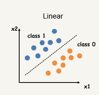
Key Question: How do we draw a line to separate the classes?

The Decision Boundary

We want to find a line (decision boundary) that separates the two classes.

Decision Boundary: \[w_1 x_1 + w_2 x_2 + w_0 = 0\]

Pass (Class 1): \(w_1 x_1 + w_2 x_2 + w_0 > 0\)
Fail (Class 0): \(w_1 x_1 + w_2 x_2 + w_0 < 0\)

In general (more than 2 features): \[w_1 x_1 + w_2 x_2 + \cdots + w_n x_n + w_0 = 0\] The model is still linear, but the boundary is a hyperplane in \(n\) dimensions.

Another Dataset Example

In practice, data is rarely perfectly separable.

Goal: Find the most general linear boundary that minimizes classification error.

Points near the boundary may be misclassified
We want the boundary that makes the fewest mistakes overall

Key insight: We need a model that outputs a confidence score (probability), not just a hard 0/1 decision.

1. Introduction✓

2. The Sigmoid Function●

3. Logistic Regression○

4. Loss Function○

5. Gradient Derivation○

6. Training○

7. One-vs-All Classification○

From Scores to Probabilities

Let \(z = w_1 x_1 + w_2 x_2 + \cdots + w_n x_n + w_0\) be the linear score.

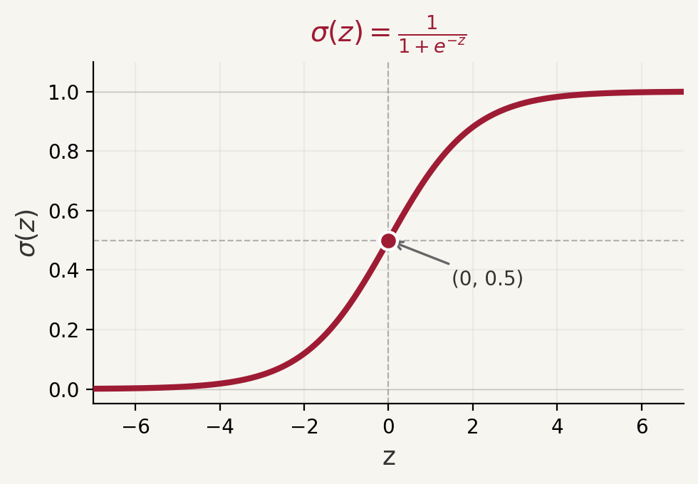
We need a function that maps \(z \in (-\infty, +\infty)\) to a probability in \([0, 1]\).

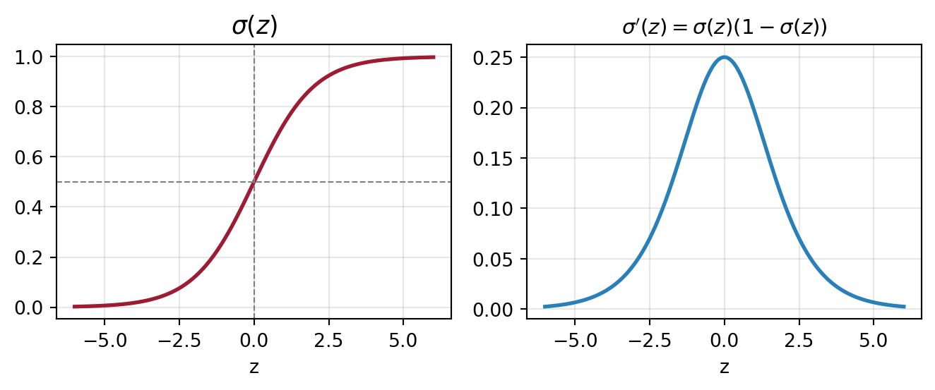
\[\sigma(z) = \frac{1}{1 + e^{-z}}\]

Input \(z\)	\(\sigma(z)\)	Interpretation
\(-\infty\)	\(0\)	Definitely Class 0
\(0\)	\(0.5\)	Uncertain
\(+\infty\)	\(1\)	Definitely Class 1

Sigmoid: Shape and Derivative

Properties of \(\sigma(z)\):

Output is always in \([0, 1]\) ✅
Smooth and differentiable everywhere ✅
Symmetric around \((0, 0.5)\)
Maps any real number to a probability

Simple and elegant derivative: \[\frac{d\sigma}{dz} = \sigma(z)\big(1 - \sigma(z)\big)\]

1. Introduction✓

2. The Sigmoid Function✓

3. Logistic Regression●

4. Loss Function○

5. Gradient Derivation○

6. Training○

7. One-vs-All Classification○

The Logistic Regression Model

Logistic Regression is a linear classifier that outputs a probability.

\[\hat{y} = \sigma(z) = \sigma\!\left(\sum_{i=0}^{n} w_i x_i\right) = \frac{1}{1 + e^{-\mathbf{w}^T \mathbf{x}}}\]

Prediction rule:

If \(\hat{y} > 0.5\) → predict Class 1 (Pass ✅)
If \(\hat{y} \leq 0.5\) → predict Class 0 (Fail ❌)

This is equivalent to: if \(z > 0\) → Class 1, if \(z \leq 0\) → Class 0.

Why “Regression”? Because the internal score \(z\) is computed via linear regression — logistic regression wraps it with a sigmoid to produce probabilities.

Example: Predicting Exam Results

Suppose the model has learned: \(\hat{y} = \sigma\!\left(x_{\text{study}} + 2\,x_{\text{sleep}} - 8\right)\)

Student	Study (\(x_1\))	Sleep (\(x_2\))	\(z\)	\(\hat{y} = \sigma(z)\)	Prediction
1	5	7	\(5+14-8=11\)	\(\approx 1.00\)	✅ Pass
2	3	8	\(3+16-8=11\)	\(\approx 1.00\)	✅ Pass
3	1	3	\(1+6-8=-1\)	\(0.269\)	❌ Fail
4	2	2	\(2+4-8=-2\)	\(0.119\)	❌ Fail

The model outputs a confidence: Student 4 has only a 11.9% chance of passing — much more informative than a hard 0/1 label!

Logistic Regression Summary

Component	Formula / Description
Linear Score	\(z = \mathbf{w}^T \mathbf{x} = w_1x_1 + \cdots + w_nx_n + w_0\)
Output (probability)	\(\hat{y} = \sigma(z) = \frac{1}{1+e^{-z}} \in [0,1]\)
Decision Boundary	\(z = 0 \;\Leftrightarrow\; \hat{y} = 0.5\)
Class 1	\(\hat{y} > 0.5\) (i.e., \(z > 0\))
Class 0	\(\hat{y} \leq 0.5\) (i.e., \(z \leq 0\))

1. Introduction✓

2. The Sigmoid Function✓

3. Logistic Regression✓

4. Loss Function●

5. Gradient Derivation○

6. Training○

7. One-vs-All Classification○

Why Not Use Squared Loss?

Since \(\hat{y} \in [0,1]\) is a probability, squared loss \((y - \hat{y})^2\) is technically valid but leads to a non-convex optimization landscape with many local minima.

We need a loss designed for probability outputs → Log Loss (Cross-Entropy Loss)

Intuition:

If \(y = 1\) and \(\hat{y} \approx 1\) → loss should be small ✅
If \(y = 1\) and \(\hat{y} \approx 0\) → loss should be large ❌
We want a function that heavily penalizes confident wrong predictions

Log Loss (Cross-Entropy Loss)

When \(y = 1\): \[\color{#2980b9}{\ell = -\log(\hat{y})}\]

\(\hat{y} \to 1\): loss \(\to 0\) ✅
\(\hat{y} \to 0\): loss \(\to \infty\) ❌

When \(y = 0\): \[ \ell = -\log(1 - \hat{y})\]

\(\hat{y} \to 0\): loss \(\to 0\) ✅
\(\hat{y} \to 1\): loss \(\to \infty\) ❌

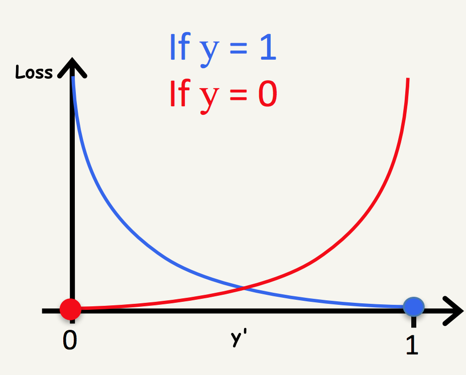
Unified: \(\quad \quad \quad \ell(y, \hat{y}) = -y\log(\hat{y}) - (1-y)\log(1-\hat{y})\)

Unified Loss Formula

\[\ell(y, \hat{y}) = -y\log(\hat{y}) - (1-y)\log(1-\hat{y})\]

Verify the formula:

When \(y=1\): \(\ell = -\log(\hat{y}) - 0 = -\log(\hat{y})\) ✅
When \(y=0\): \(\ell = 0 - \log(1-\hat{y}) = -\log(1-\hat{y})\) ✅

Over the full dataset (\(N\) examples): \[\mathcal{L} = -\frac{1}{N}\sum_{i=1}^{N}\left[y^{(i)}\log(\hat{y}^{(i)}) + (1-y^{(i)})\log(1-\hat{y}^{(i)})\right]\]

1. Introduction✓

2. The Sigmoid Function✓

3. Logistic Regression✓

4. Loss Function✓

5. Gradient Derivation●

6. Training○

7. One-vs-All Classification○

Applying the Chain Rule

We have the chain: \(w_i \xrightarrow{\;z = \mathbf{w}^T\mathbf{x}\;} z \xrightarrow{\;\sigma\;} \hat{y} \xrightarrow{\;\ell\;} \text{loss}\)

\[\frac{d\ell}{dw_i} = \frac{d\ell}{d\hat{y}} \cdot \frac{d\hat{y}}{dz} \cdot \frac{dz}{dw_i}\]

Step 1 — \(\frac{dz}{dw_i}\): \(\quad \frac{dz}{dw_i} = x_i\)

Step 2 — \(\frac{d\hat{y}}{dz}\): \(\quad \frac{d\hat{y}}{dz} = \sigma(z)(1-\sigma(z)) = \hat{y}(1-\hat{y})\)

Step 3 — \(\frac{d\ell}{d\hat{y}}\): \(\quad \frac{d\ell}{d\hat{y}} = -\frac{y}{\hat{y}} + \frac{1-y}{1-\hat{y}}\)

The Beautiful Cancellation

Putting it all together:

\[\frac{d\ell}{dw_i} = \underbrace{\left[\frac{-y}{\hat{y}} + \frac{1-y}{1-\hat{y}}\right]}_{\frac{d\ell}{d\hat{y}}} \cdot \underbrace{\hat{y}(1-\hat{y})}_{\frac{d\hat{y}}{dz}} \cdot \underbrace{x_i}_{\frac{dz}{dw_i}}\]

\[= \left[\frac{-y(1-\hat{y}) + (1-y)\hat{y}}{\hat{y}(1-\hat{y})}\right] \cdot \hat{y}(1-\hat{y}) \cdot x_i\]

\[= \left[-y + y\hat{y} + \hat{y} - y\hat{y}\right] \cdot x_i = (\hat{y} - y)\, x_i\]

\[\boxed{\frac{d\ell}{dw_i} = (\hat{y} - y)\, x_i}\]

This is identical in form to the linear regression gradient — the sigmoid derivative cancels out beautifully!

1. Introduction✓

2. The Sigmoid Function✓

3. Logistic Regression✓

4. Loss Function✓

5. Gradient Derivation✓

6. Training●

7. One-vs-All Classification○

Gradient Descent Update Rule

Gradient: \[\frac{d\ell}{dw_i} = (\hat{y} - y)\,x_i \qquad \frac{d\ell}{dw_0} = (\hat{y} - y)\]

Update rule (gradient descent): \[w_i \leftarrow w_i - \eta\,(\hat{y} - y)\,x_i \qquad w_0 \leftarrow w_0 - \eta\,(\hat{y} - y)\]

If \(\hat{y} > y\) (over-predicted) → gradient is positive → decrease weights
If \(\hat{y} < y\) (under-predicted) → gradient is negative → increase weights
If \(\hat{y} = y\) (perfect) → gradient is zero → no update

Training Algorithm

Step	Action
1	Initialize \(w_1, \ldots, w_n, w_0\) randomly (or to zero)
2	Pick a random data point \((x_1^{(i)}, \ldots, x_n^{(i)}, y^{(i)})\)
3	Compute \(z = \mathbf{w}^T\mathbf{x}^{(i)}\)
4	Compute prediction \(\hat{y}^{(i)} = \sigma(z)\)
5	Update: \(w_j \leftarrow w_j - \eta(\hat{y}^{(i)} - y^{(i)})\,x_j^{(i)}\) for all \(j\)
6	Repeat from Step 2 until convergence

Stopping rule: when the loss change per iteration falls below a threshold \(\epsilon\).

1. Introduction✓

2. The Sigmoid Function✓

3. Logistic Regression✓

4. Loss Function✓

5. Gradient Derivation✓

6. Training✓

7. One-vs-All Classification●

Extending to Multiple Classes

Logistic regression is inherently binary (two classes). For \(K\) classes, we use the One-vs-All (OvA) strategy.

Procedure:

Train \(K\) separate binary classifiers: one per class
Classifier \(k\) predicts: “Is this example Class \(k\) or not?”
Each outputs a probability \(\hat{y}_k = \sigma(z_k)\)
Predict the class with the highest probability: \[\hat{y} = \underset{k \in \{1, \ldots, K\}}{\arg\max}\; \hat{y}_k\]

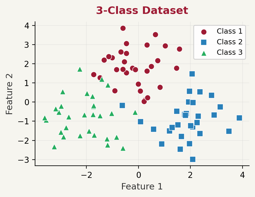
For \(K = 3\) classes: train 3 classifiers and pick the most confident one.

One-vs-All: Diagram

For \(K\) classes: \(\hat{y} = \underset{k \in \{1, \ldots, K\}}{\arg\max}\; f_k(x)\)

One-vs-All: Visualization

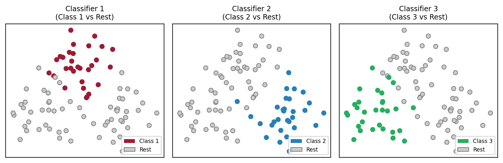
Each classifier learns to separate one class from the rest. Final answer: class with highest \(\hat{y}_k\).

Thank You!

CS-466/566: Math for AI

TABLE OF CONTENTS

Classification vs. Regression

🏷️ Classification Models

📈 Regression Models

Classification vs. Regression

Will You Pass the Exam?

📋 The Scenario

The Decision Boundary

Another Dataset Example

TABLE OF CONTENTS

From Scores to Probabilities

Sigmoid: Shape and Derivative

TABLE OF CONTENTS

The Logistic Regression Model

Example: Predicting Exam Results

Logistic Regression Summary

TABLE OF CONTENTS

Why Not Use Squared Loss?

Log Loss (Cross-Entropy Loss)

Unified Loss Formula

TABLE OF CONTENTS

Applying the Chain Rule

The Beautiful Cancellation

TABLE OF CONTENTS

Gradient Descent Update Rule

Training Algorithm

TABLE OF CONTENTS

Extending to Multiple Classes

One-vs-All: Diagram

One-vs-All: Visualization

Thank You!